Optimal Transport: Wasserstein distance and Sinkhorn
The goal of optimal transport problems, is to find optimal mappings between probability meaures: these mappings are also called transport plans, and can take the form of functional transforms (in Monge's original problem) or joint probability distributions (in the Kantorovitch relaxation).
OT formulations have found practical applications in imaging, notably in histogram equalization, in machine learning (for distribution matching), and also in the study of partial differential equations (see the work of Villani, Ambrosio, Benamou and Brenier). The first two sets of applications have grown from the development of efficient numerical solvers.
In this blog post I will quickly summarize what OT problems, and introduce a simple, efficient algorithm that is able to solve quite a few problems and can have quite a few extensions.
Let \( \mu_0, \mu_1 \) be probability measures on the spaces \( \mathcal{X} \) and \( \mathcal{Y} \), and \( c: \mathcal{X}\times\mathcal{Y}\to \RR \) be a cost function on the product space.
$$ \begin{equation} \begin{aligned} &\inf_\gamma \int_{X\times Y} c(x,y) d\gamma \ &\suchthat P^1_{#}\gamma = \mu, P^2_{#}\gamma = \nu. \end{aligned} \end{equation} $$
Notice that the constraint by which \( \gamma \) is a probability measure summing to \( 1 \) is implied by the constraint that its marginals are the problem data \( \mu, \nu \). The latter constraint is also called the coupling constraint.
In the case where \( \mathcal{X} = \mathcal{Y} \), the value of the minimum is called the Wasserstein or Kantorovitch-Rubinstein distance and is denoted \( \mathcal{W}(\mu, \nu) \) -- it is a distance function of the space of probability measures \( \mathcal{M}^1(\mathcal{X}) \).
Generalizations exist, such as the multi-marginal case, where the transport problem pertains to multiple measures \( \mu_k \). These can have interesting links to energy minimization schemes and graphical models.
Discrete measures
A large class of numerical algorithms cover cases where the measures are discrete, of the form \( \mu = \sum_{i=0}^n \mu^i \delta_{x_i} \). This case also represents histograms, where the \( x_i \) correspond to the histogram bins. Applying these methods to continuous-space problems (with density-based measures for instance) involves intermediary steps such as grid discretization and binning, although other methods for these problems can instead rely on using basis functions
In the latter case, any joint distribution coupling \( \mu \) and \( \nu \) is of the form \( \gamma = \sum_{i,j} \gamma^{ij}\delta_{(x_i,y_j)} \), and denoting \( \mathbf{C} = (c(x_i,y_j))_{i,j} \). The transport problem reads
$$ \begin{aligned} \inf_{\gamma}{}& \langle \mathbf{C}, \gamma \rangle \ \suchthat &\gamma \mathbf{1} = \mu \ &\gamma^\top\mathbf{1} = \nu, \end{aligned} $$
where \( \langle \cdot,\cdot\rangle \) is the Frobenius inner product.
In this form, we see that the OT problem is merely a (high-dimensional) linear program (LP) with linear equality constraints, which can be solved efficiently using standard algorithms, namely Dantzig's simplex algorithm.
Popular packages for this are included in Google's Glop included in OR-Tools, or the Gurobi suite of solvers, and of course scipy comes with its own LP module.
Enhancing methods for linear programming is still an active research domain, covering everything from dualization methods, interior point algorithms, or even making Dantzig's classic method more robust.
OT at scale: the Sinkhorn algorithm
For large-scale problems, using an LP solver, relying on the simplex method for instance, implies high computational cost. Relaxation techniques have to be used, and the more suited to the nature of the problem (mass transport between probability measures), the better. Cuturi [2] proposes a relaxation of the form
$$ \begin{equation} \inf \int_{\mathcal{X}\times \mathcal{Y}} c(x,y)d\gamma - \epsilon H(\gamma), \end{equation} $$
where \( H(p) = -\int (\log p(x) - 1)dp(x) \) is the entropy of measure \( p \).
Introducing the problem Lagrangian with Lagrange multipliers \( \alpha, \beta \) (also called dual potentials), we find that the optimal transport plan reads
$$ \gamma^\star_{ij} = \exp(-(C_{i,j} + \alpha_i + \beta_j)/\epsilon), $$
with optimal Lagrange multipliers satisfying
$$ \begin{equation}\label{eq:SinkhornFixedPoint} u = \frac{\mu}{Kv} \quad v = \frac{\nu}{K^\top u} \end{equation} $$
where \( K = \exp(-\mathbf{C}/\epsilon) \) and \( (u,v) = (\exp(-\alpha/\epsilon), \exp(-\beta/\epsilon)) \).
The optimal transport plan is then recovered from \( \gamma^\star_{i,j} = u_i K_{i,j}v_j \), or \( \gamma = K\odot (u \otimes v) \). Sinkhorn iterations consist in solving the fixed-point mapping above iteratively. The minimizer is often denoted \( \calW_\epsilon(\mu, \nu) \) and is called the Sinkhorn distance.
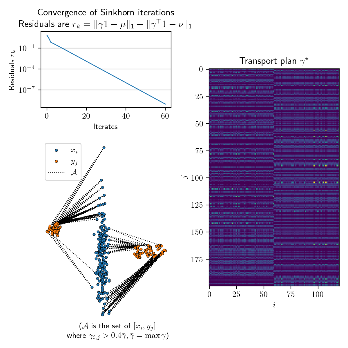
An important detail is how convergence is tested. One can test the value of the multipliers converges within some given tolerance \( \tau > 0 \) -- but this convergence criterion is sensitive to the choice of regularization \( \epsilon \). A better alternative is checking for primal feasibility, i.e. compliance with the constraints, which read \( u\odot Kv = \mu \) and \( v\odot K^\top u = \nu \) in terms of the dual variables. $$ \begin{equation} | u\odot Kv - \mu |_1 + | v\odot K^\top u - \nu |_1 \leq \tau. \end{equation} $$ Using the form above is more computationally efficient than recomputing \( \gamma \) at every iteration and checking for \( \gamma \mathbf{1}=\mu \).
Here is a basic, 20-line implementation of the Sinkhorn distance:
def sinkhorn(mu, nu, C, eps):
    u = np.zeros_like(mu)
    v = np.empty_like(nu)
    K = np.exp(-C/eps)
    thresh = 1e-9
    max_iter = 4000
    ress_ = []
    for t in range(max_iter):
        u[:] = mu / (K @ v)

        ktu = K.T @ u
        r = v * ktu
        v[:] = nu / ktu
        s = u * (K @ v)
        res_mu = sum(abs(s - mu))
        res_nu = sum(abs(r - nu))
        res = res_mu + res_nu
        ress_.append(res)
        if res < thresh:
            break
    P_opt = np.diag(u) @ K @ np.diag(v)
    return P_opt, u, v, ress_
More details about the algorithm are available in the reference book by Peyré and Cuturi [1], in chapter 4. But let's elaborate on a possible interpretation of the algorithm as a proximal-point method.
Introducing the so-called Gibbs matrix \( K \) into the regularized OT objective, we see that it can be rewritten as the Kullback-Leibler projection of \( K \) onto the coupling constraint:
$$ \begin{equation} \begin{aligned} &\inf_\gamma \KL(\gamma | K)\ &\suchthat \gamma\mathbf{1} = \mu, \gamma^\top\mathbf{1} = \nu, \end{aligned} \end{equation} $$ where \( \KL(P|K) = \sum_{i,j} \log(\frac{P_{i,j}}{K_{i,j}})P_{i,j} \).
Below is an example, where we compute optimal transport between two discrete distributions sampled from a multivariate Gaussian (in blue) and a mixture of Gaussians (in orange).
Pain points: optimizing the algorithm
Problems due to dimensionality of the problem still arise within the Sinkhorn iterations themselves: at each iteration, 2 matrix-vector products have to be computed, which has complexity \( \mathcal{O}(nm \max(n,m)) \).
One first optimization is to look for efficient ways to compute this matrix vector product. Depending on the structure of the cost function, we might get a factorization of the Gibbs matrix in the form \( K_1K_2 \), where the \( K_i \) might have a sparsity pattern.
An important case is when the cost is a separable function in some block coordinates of the points \( x = (x^1, \ldots, x^K) \), such that $$ c(x, y) = \sum_{s=1}^M c_s(x^s, y^s) $$ then \(K \) is separable with each factor operating only on the subspace corresponding to the \(s\) -th coordinate (then, \( K \) can be rewritten as a tensor product).
[1, chap. 4] gives a classical example for the Gaussian Gibbs kernel \( K_{i,j} = e^{-\frac{1}{\epsilon}|x_i-y_j|^2} \) (associated with using the Euclidean distance as a ground cost), which has direct applications to working with images -- and has a link to Gaussian filtering.
Another aspect is numerical stability. The classic trick of adding a small floating point number (close to floating point precision) in \eqref{eq:SinkhornFixedPoint} to avoid dividing by zero still applies. For additional robustness, one can use the logsumexp trick to instead carry out the updates in the log-domain.
Conclusion
The field of OT is incredibly rich, whether it be its theory, generalizations or applications, which is also reflected in how methods to solve OT problems connect to other subjects in mathematical optimization. This blog post merely scratched the surface. I cannot enough recommend Peyré and Cuturi's book Computational Optimal Transport [1], which is an easy read and a fantastic reference for anyone looking to learn more from a practicioner's perspective. It is further supported by the companion numerical tours, which cover some of the aforementioned applications and algorithms (notably log-domain Sinkhorn).
- [1] Gabriel Peyré, Marco Cuturi, Computational Optimal Transport. https://optimaltransport.github.io/book/
- [2] Marco Cuturi, Sinkhorn Distances: Lightspeed Computation of Optimal Transport, NeurIPS 2013. http://marcocuturi.net/Papers/cuturi13sinkhorn.pdf